Early Technologies for Image Generation

Introduction

  Before modern generative models like GANs, VAEs, and diffusion models, researchers had already developed many different ways to create images. These older approaches may look simple today, but they each introduced important ideas that shaped the field of generative modeling.

  Most of these early models focused on patterns, textures, and small images, because computers were slow and memory was limited. Some models tried to memorize patterns and retrieve them when needed, while others tried to sample images by following probabilistic rules. A few methods didn’t learn parameters at all, they simply used clever ways of copying or assembling pieces of existing images to make new ones.

  In this article, we will look at major early image generation methods. Each one represents a different idea about how images are formed and how they can be recreated from associative memories and energy-based models, to texture synthesis and early statistical approaches. Together, they form the foundation on which today’s generative AI models were built.

1. Hopfield Networks (1982)

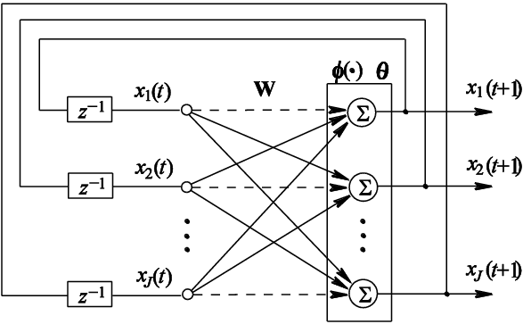
  A Hopfield network is a form of neural network that serves as an associative memory system. It consists of binary neurons with symmetric connections and no self-loops, and it evolves by updating neurons to reduce an energy function. Hopfield showed that by setting the weights appropriately (using a Hebbian rule), the network can store a set of binary patterns as stable attractors. If you present a noisy or partial version of a stored image, the network’s dynamics will iteratively recall the nearest stored image, i.e. settle into the closest attractor pattern. This demonstrated one of the first neural models of content-addressable memory for images.

  Historically, Hopfield networks (introduced by John Hopfield in 1982) were significant as they bridged physics and neural computation. Hopfield interpreted neuron states as spins and the weight matrix as interaction energies. The model sparked interest in using energy minima for computation and showed how a network could auto-associate patterns, a key early milestone in generative image modeling. However, Hopfield nets have limited storage capacity (about 0.14× number of neurons patterns) and can only regenerate images already stored (no novel samples), sometimes getting stuck in spurious memories. Despite these limits, they established the idea of using recurrent networks to generate or restore images.

  Although Hopfield networks do not generate new images in the modern sense, they introduced the key idea that a neural system could store visual patterns as attractors and recover them through internal dynamics. This made them an important conceptual predecessor to later generative models: they showed that images could be represented as stable states of an energy function and that a model could “produce” an image by evolving its internal state toward a learned pattern. This shift from classification to memory-based reconstruction helped pave the way for energy-based and generative approaches that would eventually learn to create entirely novel images.

---

2. Boltzmann Machines / Restricted Boltzmann Machines (RBMs) (1985–1995)

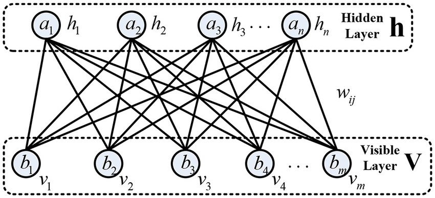
  A Boltzmann machine is another early generative neural network, introduced by Hinton and Sejnowski in 1985. It’s essentially a stochastic Hopfield network: neurons are binary but update probabilistically according to a Boltzmann distribution. Boltzmann machines (BMs) contain “visible” units (data) and can include “hidden” units to model complex dependencies. They learn by adjusting weights so that the generated distribution gets closer and closer to the training data distribution. In practice, this was very slow, but the significance was that BMs provided a probabilistic generative model, one could in principle sample the network to generate new data patterns.

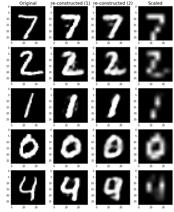
  Restricted Boltzmann Machines (RBMs) are a simplified version where no intra-layer connections exist (only bipartite connections between visible and hidden units). This restriction (introduced by Smolensky and Hinton in the late 1980s–1990s) allows efficient block Gibbs sampling⁽¹⁾ and training (especially with Hinton’s Contrastive Divergence algorithm around 2002). An RBM defines a probability distribution over binary images via an energy function. Once trained on images, an RBM can produce new samples by an alternating Gibbs sampling of hidden and visible units (letting the network “dream” new images). For example, an RBM trained on handwritten digits will generate digit-like patterns when sampled. In one experiment, an RBM trained on MNIST digits produced novel outputs, some looked like distorted or blended digits. This shows how the RBM doesn’t just memorize training samples but learns a distribution and can generate new images from it.

  Historically, Boltzmann machines were important as one of the first approaches to statistically model images with neural networks. They introduced concepts like using hidden units to capture higher-order correlations and using sampling-based learning. However, early BMs were limited to very small images or simplistic patterns. The advent of RBMs (and faster learning) in the mid-199s revitalized this approach. RBMs became the building blocks of deeper models (as in Deep Belief Nets). They demonstrated that even a single-layer network could learn a distribution over, say, 28×28 pixel digit images and stochastically generate plausible digit-like outputs. This was a stepping stone between early energy-based models and later large-scale generative models.

---

3. Deep Belief Networks (DBNs) (2006)

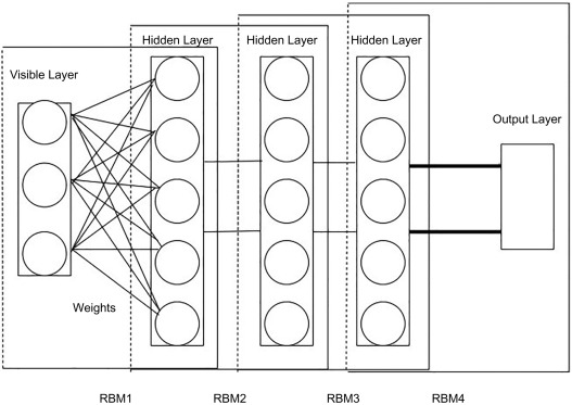
  Deep Belief Networks are multilayer generative models that stack simple generative modules (like RBMs) into a deep architecture. Hinton et al. introduced DBNs in 2006 as a way to efficiently train deep neural networks. A DBN is composed of multiple layers of hidden units, where each pair of adjacent layers forms an RBM (an undirected bipartite model), except the top layers which together form a joint Boltzmann machine. By training greedily layer by layer (each layer of features is trained to model the activations of the layer below), the DBN learns a hierarchical generative model. After training, one can generate an image by first sampling the top-layer RBM, then propagating those samples downward (layer by layer) to the visible units.

  Conceptually, a DBN learns abstract features in higher layers that generate more concrete details in lower layers. For example, in a DBN trained on handwritten digits, the top layer might represent high-level “which digit” features, and the lower layers generate strokes and pixels. Historically, DBNs were significant because they demonstrated the first effective strategy to train deep neural networks (before modern backpropagation was fully successful for very deep nets). They sparked the deep learning renaissance by showing that multiple layers of latent variables could be learned and that these models could generate recognizable images (not just classify them). In Hinton’s 2006 work, a DBN was trained on the MNIST dataset. When sampling from the model, it would generate images that “look like real digits of all classes.”

  One reliable example is a DBN trained on a dataset of handwritten digits: after training, by initializing the top-layer units randomly and “unrolling” the generative process, the network could produce synthetic digit images (some 0–9 digits that never appeared in training). These images were often somewhat blurry or distorted (since the model still had limited capacity), but recognizably digits. The DBN’s ability to sample across all classes (0–9) highlighted that it had learned a global model of the data, as opposed to memorizing specific examples. This success was historically important,it showed deep networks could be generative and not just discriminative. Moreover, DBNs (and their later refinement, Deep Boltzmann Machines) were forerunners to modern deep generative approaches, illustrating the power of layerwise learning of features. In summary, DBNs were a key evolutionary step, combining ideas from RBMs and Bayesian networks to build deeper image generators. They confirmed that depth improves generative modeling, as the higher-layer features helped capture more complex structure than a single-layer model.

---

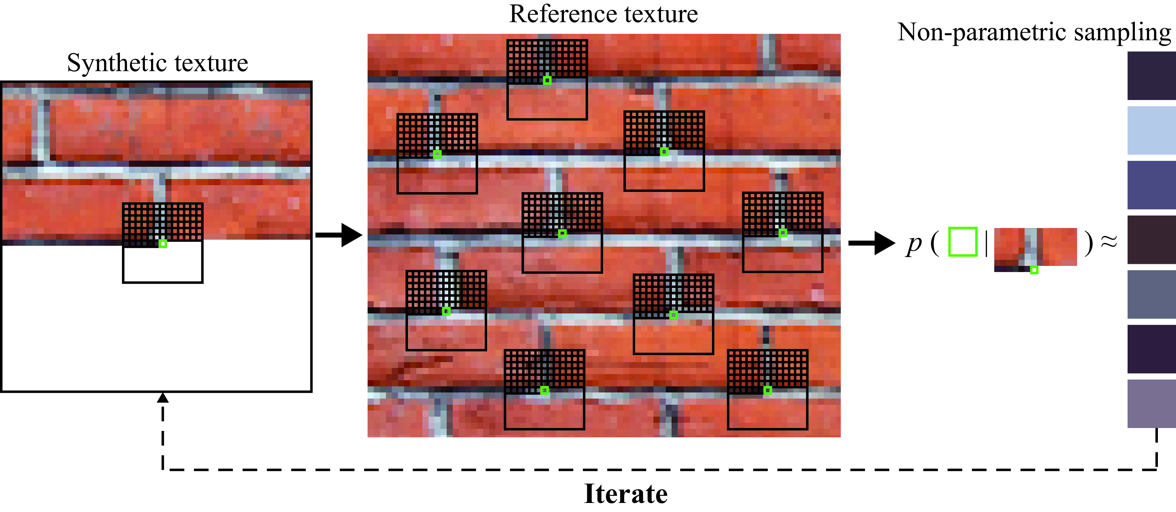
4. Non-Parametric Texture Synthesis (Efros & Leung, 1999)

  This approach, introduced by Efros and Leung in 1999, is an example-based image generation technique that does not explicitly learn global parameters. Instead, it generates a new image by sampling pixels directly from an input sample image using local conditional distributions. In the Efros-Leung algorithm, one provides a small exemplar image (e.g. a 100×100 texture sample), and the algorithm grows a larger texture outwards one pixel at a time. At each step, it considers the already-synthesized neighbors of the new pixel and searches the exemplar for similar neighborhoods. It then randomly picks one matching neighborhood from the exemplar and uses that neighborhood’s center pixel as the new pixel value. In effect, it copies local patterns from the source texture wherever they statistically match the target neighborhood, thereby building an output that preserves local texture structure without an explicit global model.

  Historically, this was a breakthrough because prior texture synthesis methods were largely parametric. Efros & Leung’s non-parametric sampler was simple yet produced impressively realistic results for many natural textures. It demonstrated that one could avoid complex parameter estimation and still generate new imagery by leveraging the source image data directly (“texture by example”). This method sparked a whole class of example-based synthesis techniques in the early 2000s, including improvements like faster patch-based methods. It was significant in the evolution of generative modeling as it shifted focus from analytical models to data-driven approaches. Essentially, the algorithm embodies a Markov random field assumption: the probability of a pixel can be determined by a small patch of its neighbors. By sampling from the exemplar’s actual patches, it sidesteps the need to explicitly model that distribution.

  The non-parametric texture synthesis method proved very effective for stochastic or semi-regular textures (brick walls, tree bark, fabric etc.). It did sometimes produce quirks, for instance, occasional visual seams or odd elements (“garbage patches” if the matching tolerance was too high). But overall it was qualitatively better than earlier methods at preserving natural detail. Its legacy is seen in later work like “image quilting” and even neural style transfer (which similarly copies patches/activations from examples). Importantly, Efros & Leung showed that to generate a realistic texture, one can rely on copying actual neighborhoods from real images, a concept underlying many modern patch-based and example-based image generation techniques.

---

5. Markov Random Field (MRF) Texture Models (1980s–2000s)

  Before modern methods that generate textures by copying existing image patches, the Markov Random Field (MRF) was the leading approach. An MRF is a probabilistic model where an image is treated as a grid of pixels, and the color of any one pixel depends only on its immediate neighbors (the Markov Property). To define a specific texture, researchers specify local clique potentials (rules that assign a score or energy to small groups of neighboring pixels). An image configuration that follows these rules well (e.g., adjacent pixels are similar for a smooth texture) will have low energy and a high probability according to the Gibbs distribution. By using iterative techniques like Gibbs sampling, the model generates new, synthetic images that gradually emerge from random noise. The process works by constantly updating each pixel based on the learned local rules until the entire image reaches equilibrium, resulting in a novel sample that statistically matches the local properties of the original training texture.

  Historically, MRFs were crucial because they provided one of the first reliable, mathematical methods to create synthetic images by treating the image as a sample drawn from a specific probability distribution. This foundational idea was inspired by early texture studies, like those by Julesz. Later models, such as the FRAME model (1997), were essentially MRFs that used complex rules (clique potentials) based on statistics from specialized image processors to synthesize remarkably realistic textures. However, MRFs had a major drawback: the generation process, which uses iterative techniques like Gibbs sampling, was extremely slow. It often took hours to produce a high-quality texture, could get stuck in non-optimal patterns, or produce unwanted repeating artifacts, a problem later addressed by faster, non-parametric methods.

  Compared to the later non-parametric method of Efros & Leung, MRF-based texture models explicitly learn a global probabilistic model and rely on slow iterative sampling to produce an image, while Efros–Leung avoids learning altogether and simply copies real patches from the exemplar. In other words, MRFs model the distribution and then sample from it, whereas Efros–Leung bypasses modeling and directly reuses observed neighborhoods. This makes MRFs more principled but far slower and more prone to getting stuck in bad local minima, while the non-parametric approach is much faster and often produces more visually convincing textures in practice.

---

6. PCA + Sampling (Eigenfaces, 1991–1993)

  Using Principal Component Analysis (PCA) for image generation came about in the early 1990s, notably with the Eigenfaces technique by Sirovich & Kirby (1990) and Turk & Pentland (1991). The idea was to treat images (for example, faces) as high-dimensional vectors and compute the principal components, essentially, find an orthonormal basis of “eigen-images” that capture the main variance across a training set of images. Once you have these eigen-images (eigenfaces for faces), any training image can be approximated by a linear combination of a small number of them. More importantly for generation: one can sample new combinations of these basis images by choosing random coefficients (for example, sampling from a Gaussian distribution fitted to the coefficient distributions of the training data) and then adding them up to produce a new image. In essence, PCA gives a low-dimensional latent space (spanned by eigenfaces) and one can generate novel images by picking a random point in that space.

  In the context of faces, this produces ghostly, average-looking faces. Historically, this was one of the first demonstrations of data-driven image generation: researchers showed that by randomly sampling in “face space,” you could create a face that looks human-like though it never belonged to a real person. These faces were usually blurry and lacked fine detail (since only the largest few principal components were used), but they did capture high-level attributes like general face shape, hair darkness, etc. This underscores that while not photo-realistic, the linear model could produce recognizable new faces. The generated images tended to be somewhat like an “average” face plus some variation, if too much variation was added (e.g., using full range of coefficients), the face could look bizarre (distorted features), because the linear model doesn’t capture non-linear constraints like “eyes should be symmetric.”

Conclusion

  Together, these early image-generation methods show how the field evolved long before today’s deep models. Each approach, whether based on associative memories, probabilistic sampling, linear subspaces, or example-based synthesis captured a different intuition about how images are structured and how they can be recreated. None of them produced high-resolution or fully novel images as modern GANs, VAEs, or diffusion models do, but they introduced the core ideas that made those later breakthroughs possible: learning distributions, using latent representations, modeling local dependencies, and reconstructing data from internal rules. By tracing these foundations, we can better appreciate how today’s generative AI stands on decades of creative and diverse work in image modeling.

---